
In a time when data is like digital gold, being able to efficiently navigate and work with large datasets is a fundamental skill in almost every professional field. One of the most useful features of Google Sheets, a crucial part of Google's extensive office suite, is VLOOKUP, which has the potential to completely transform data processing. The integration of VLOOKUP into your Google Sheets workflow, alongside the ability to integrate Google Sheets with various other applications and platforms, allows for a seamless blend of data retrieval, management, and analysis, enhancing productivity. The purpose of this guide is to provide a clear path to mastering VLOOKUP in Google Sheets by explaining its subtleties and demonstrating how to integrate this powerful tool, as well as integrate Google Sheets itself, effectively into your data analysis tasks.
What is VLOOKUP?
VLOOKUP, an acronym for Vertical Lookup, is a highly functional and versatile tool within Google Sheets and other spreadsheet software. It serves as an essential function for anyone working with large sets of data, offering a streamlined approach to data retrieval. At its core, VLOOKUP is designed to search vertically down the first column of a specified range for a particular value. Once it locates this value, it returns a corresponding value from another column in the same row. The real power of VLOOKUP lies in its simplicity coupled with its robust functionality. Whether you’re dealing with extensive databases, complex financial records, or any sizable dataset, VLOOKUP is engineered to swiftly navigate through the data. This functionality not only saves time but also significantly reduces the margin for error that comes with manual data searching.What is the Syntax of the VLOOKUP Formula?
The syntax of the VLOOKUP formula is a structured format that defines how the function should be written to work correctly in spreadsheet software like Google Sheets or Microsoft Excel. The standard syntax of the VLOOKUP formula is:=VLOOKUP(search_key, range, index, [is_sorted])Here's a breakdown of each component in this syntax:
- search_key: This is the value you are searching for in the first column of your specified range. It's the item you want to look up. The search key can be a specific value, text, number, or a reference to a cell containing the value.
- range: This refers to the cell range where the search will take place. It includes the column containing the search key and the columns from which you want to retrieve data. It's important to note that VLOOKUP will only look for the search key in the first column of this range.
- index: This is the column index number from the range you specified from which to return a value. For instance, if the range is A2:B10, and you want to return a value from the second column (column B), your index would be 2. The index count starts from the first column of the range you specified.
- [is_sorted]: This is an optional argument, which can be either TRUE or FALSE. If TRUE (or if this argument is omitted), VLOOKUP assumes that the first column in the range is sorted in ascending order and will return the closest match to the search key. If FALSE, VLOOKUP will search for an exact match to the search key. If an exact match is not found, the function will return an error.
=VLOOKUP(search_key,SheetName!range, index, [is_sorted])How to Use VLOOKUP in Google Sheets?
Using VLOOKUP in Google Sheets is a straightforward yet powerful way to search for data in a spreadsheet. Here’s how you can effectively use VLOOKUP in your Google Sheets:Step 1: Understand Your Data
Organize Your Spreadsheet: Ensure your data is organized with the column you want to search (lookup column) as the first column of your data range. For example, if you're looking up a product ID to find its price, the product ID should be in the first column.Step 2: Identify the Lookup Value
Choose the Value You Want to Find: This is the value you will search for in the first column of your data range. It could be text, a number, or a cell reference.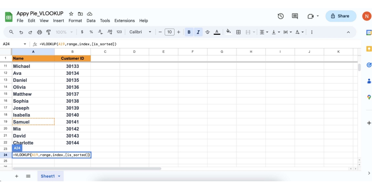
Step 3: Define the Data Range
Select the Range of Cells to Search: This range should include the lookup column and the column containing the data you want to retrieve. For instance, if your data is in columns A to B, and your lookup column is A, your range is A: B.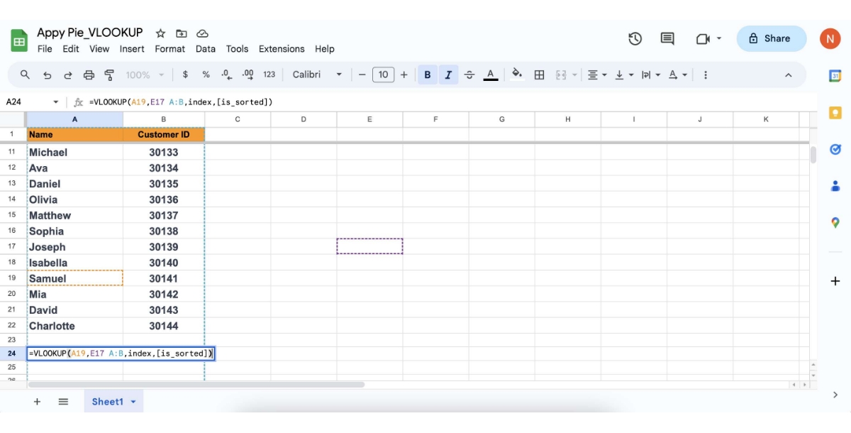
Step 4: Determine the Column Index Number
Identify the Column to Retrieve Data From: This is the number of the column within your range that contains the data you want to pull. For example, if the data you want is in the third column of your range, your index number is 2.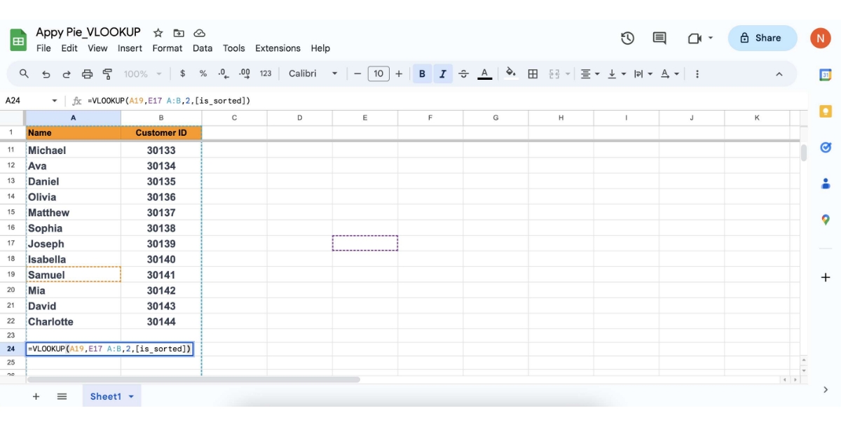
Step 5: Decide on Range Lookup
Set the is_sorted value: In our example, the data isn't sorted in order, so we'll need to use FALSE for [is_sorted].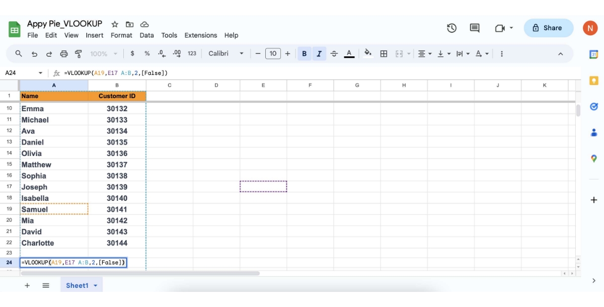
Step 6: Press Enter and Analyze the Result
Put the function into action: Press Enter after you've typed all of your input. If everything is as it should be, the function should return the desired value. Samuel's customer ID number, 30141, was returned in our instance.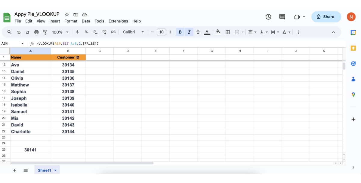 Absolutely, you've identified some of the common errors encountered while using VLOOKUP in spreadsheet applications like Google Sheets. Let's delve a bit deeper into these errors and understand their causes:
- #N/A Error
- Check the Search Key: Ensure that the search key exactly matches one of the entries in the first column. Remember, VLOOKUP is case-sensitive.
- Examine Data Formatting: Sometimes, differences in data formatting (like a number formatted as text) can cause this error.
- Verify Range Selection: Make sure the range includes the column that contains your search key.
- #REF Error
- Correct Index Number: Adjust the index number to a value within the range's width. For instance, if your range is A:D, the index number should be between 1 and 4.
- Incorrect Data
- Sort Data: If using TRUE for is_sorted, sort the first column in ascending order.
- Use FALSE for Exact Match: To avoid approximate matches, use FALSE for is_sorted. This ensures VLOOKUP only returns a value if it finds an exact match.
Cause: This error primarily occurs when VLOOKUP cannot find the search key in the first column of the specified range.Solutions:
Cause: This error appears when the column index number specified in the VLOOKUP formula is greater than the number of columns in the range.Solutions:
Cause: This issue arises when you use TRUE for the is_sorted argument while the first column of your range is not sorted in ascending order. VLOOKUP with TRUE for is_sorted looks for an approximate match and might return incorrect data if the column isn't properly sorted.Solutions:
Enhancing Google Sheets Efficiency with Appy Pie Connect
Take your Google Sheets usage to the next level by optimizing its functionality with Appy Pie Connect. This integration enables users to streamline their workflows effectively, enhancing productivity and performance in Google Sheets. Discover the possibilities with Google Sheets and Appy Pie Connect integration:
- Add rows to Google Sheets when new Trello cards are moved to a list
- Send Slack messages whenever Google Sheets rows are updated
- Create Trello cards from new rows on Google Sheets
- Add new Facebook Lead Ads leads to rows on Google Sheets
- Generate Google Calendar events from new Google Sheets rows
- Create rows in Google Sheets for new Gravity Forms submissions
- Send emails via Gmail when Google Sheets rows are updated
- Send Gmail emails for new Google Sheet spreadsheet rows
- Add new GitHub issues to Google Sheets spreadsheet rows
- Create Google Sheets rows from new scheduled Calendly events
- Add new paid Shopify orders to Google Sheets rows
- Create custom Salesforce objects from new rows on Google Sheets
Conclusion
Becoming proficient with VLOOKUP in Google Sheets is an important ability in today's data-driven society. It improves the capacity to handle big datasets effectively, making the process of processing and retrieving data easier to handle. We've gone over the nuances of VLOOKUP in this tutorial, covering everything from its fundamental syntax to real-world applications, and we've also fixed frequent mistakes to guarantee better functionality. Additionally, combining Appy Pie Connect with Google Sheets opens up a world of possibilities and allows for workflow automation that will completely change the way you work. In addition to saving time, this integration guarantees accuracy and consistency across different applications. Adopting these Google Sheets tools and methods will surely result in more streamlined, effective, and error-free data management, which will be priceless in any professional context.Related Articles
- 200+ Tasteful Food Business Name Ideas
- Customer Expectations: Types, Management Tips, and Examples
- How to Automatically Share New YouTube Videos on Discord
- How to Write a Resignation Letter? [With Resignation Letter Samples]
- Chatbots vs Virtual Assistants [Differences, Similarities, and Benefits]
- What is social selling and how it works? A step-by-step guide
- A Brief Guide To Video Marketing for Businesses in 2021
- 15 Best Character AI Alternatives & Competitors in 2023
- Top 13 Freshworks Alternatives in 2023
- Mastering PowerPoint Online: Ultimate Guide to Create & Present Dynamic Slideshows