How to Create a Pivot Table in Excel Online – A Free Guide

Do you work with data in Excel? Are you using Pivot Tables? If you are not, it is because you do not know-how. The concept of Pivot Tables has changed a lot since they were introduced, but with a new version of Excel, Microsoft has introduced modifications to the method of creating them.

What does a Pivot Table do?

It organizes the data you have in a spreadsheet and presents it in a summarised form. For instance, you may have a spreadsheet including 1000 lines of data, that can be grouped in various ways (by invoice, by the customer, by month, by city, etc.) a Pivot can show you a summary of your data by those attributes. You can add to or edit the base data in the spreadsheet, and then refresh the Pivot and a new summary will be shown indicating the updated data.

How to create a Pivot Table in Excel Online

Here is how you can create a Pivot Table in Excel Online:

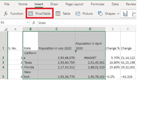
•  Go to the Excel Online spreadsheet and choose the cells including the data you want to look at.
• Choose the ‘Insert’ option and then select the ‘Pivot Table’ option.
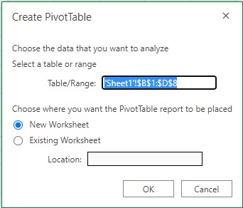
• From the pop-up, choose the ‘New Workbook’ option and then click on the ‘OK button.
• In the pivot table editor, drag the columns and rows that you want to summarize to the appropriate box.
• You can choose the fields that contain the values you want to calculate or add from the ‘Values’ section.
• You can use the ‘Filters’ section if you just want to display values that suit specific criteria.

Create the Pivot Table

The first thing that you have to do is summarize the data into a pivot table. It is suggested to name the columns before starting. Next, select the cells that include data, and from the toolbar, choose the ‘Insert’ option and then click on the Pivot Table.

A new pivot table box will pop up. It will show you the table data that you have selected and also provide you the choice of creating a pivot table in a new worksheet or the same old one. To keep it simple, it is best to select the ‘New Worksheet’ option and then click on the ‘OK button.

A new worksheet will be created where you can create your dynamic pivot table reports.

How to build a Pivot Table Report

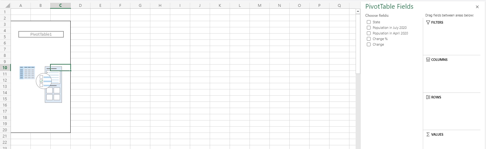
When you start, a pivot table is empty. On the right side of the sheet, you will see a pivot table editor, where you can find all the choices for creating your pivot table.
Further, the pivot table editor is divided into 2 horizontal sections:
The top section includes all the necessary fields, like the columns from your table data.
The bottom section includes the real area for using the pivot table. It also has 4 parts, columns, rows, values, and filters.

The pivot table in Excel Online makes use of drag and drop functionality. Simply by dragging it to the place you want, you can add a field to an area. If you do not want to put a field in a box anymore, you can drag it out and it will disappear. Other than this, you will learn about the rest of the tools as we move forward.

The rows, columns, values, and filters in the pivot fields are:

• The rows and columns will help to create the basic two-dimensional data from which you will calculate the third dimension of values.
• The values will help to convert text that appears in a recognized format, for instance, date, number, or time format into a numeric value.
• The filter will help to sort out the data.

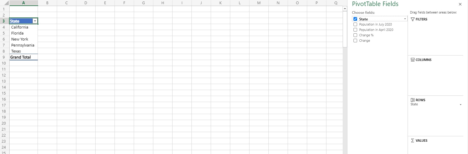
Add rows
Let us begin by adding the State Name field to the ‘Rows’ section. There are certain ways of doing it, but the best way to move ahead is by using the drag and drop feature. You need to hold on to the state name field and then move it to the ‘Rows’ section in the bottom half of the sidebar, and then release it.

Add columns
Here we have taken population in July 2020 to add in the column section. As stated above, you just have to drag the Population in July 2020 field to the columns section at the bottom of the pivot table editor.

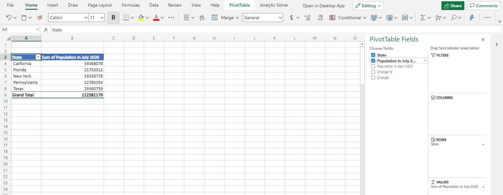
Add values
Here you need to add values to the table. You will see that a total section is created automatically.

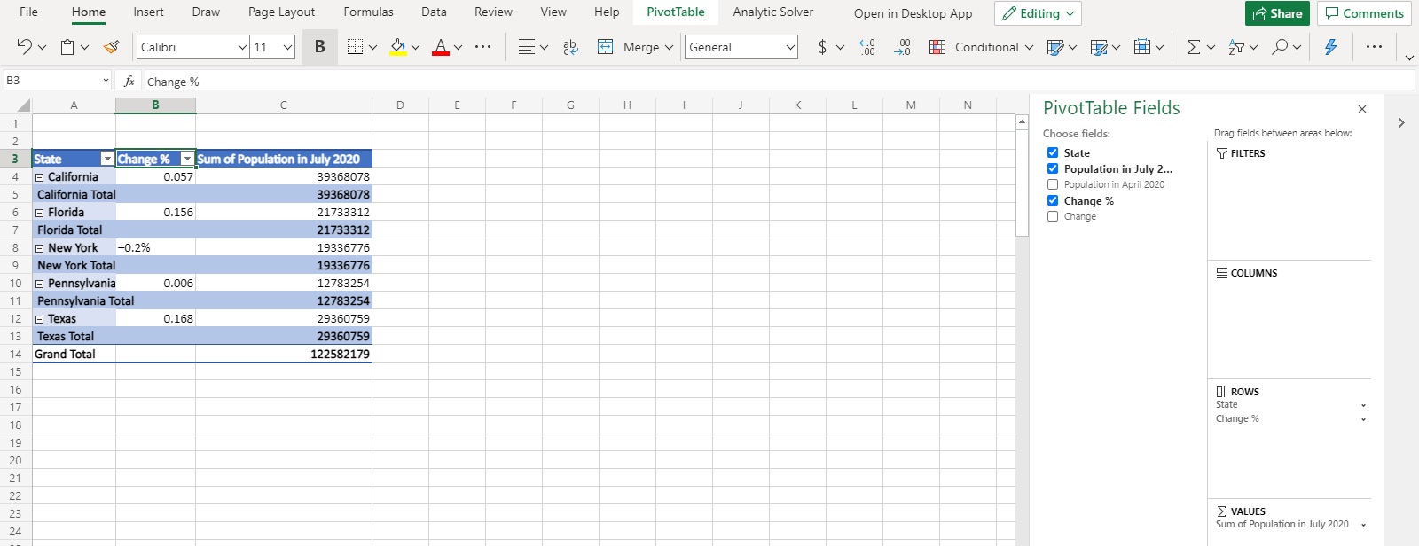
Add filters
You also need to filter the data to the values inserted. For the same, you need to drag the change field to the filters section. You will see 2 new cells at the top of the sheet.

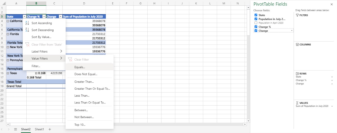You can also filter every column from the original data set.

With Appy Pie Connect, you can integrate Excel other apps to automate tedious & repetitive tasks in no time. With the Appy Pie Connect and Excel integration, you can share your spreadsheets with other stakeholders & team members.