The Ultimate Guide to Using Conditional Formatting in Google.

Spreadsheets can store large amounts of data in a single place. While you can use pivot tables to summarize that data, you cannot gain insight into the data. If you want to gain some insight just by glancing at your sheet, conditional formatting can provide you with that insight.

Conditional formatting allows you to highlight cells according to certain criteria. It can help users better understand spreadsheets at a glance and create more readable spreadsheets. The formatting can also serve as a great way to track goals, giving you visual indications of how you're progressing against specific metrics.

What Is Conditional Formatting?

Conditional formatting in Google Sheets allows you to change the aspect of a cell-based on rules you set. You can change a cell's background color or the style of the cell's text. Every rule you set is an if/then statement. All rules follow the same structure, however, some elements need to be defined:

• Range: Range defines which cell or cells the rule should apply to.
• If cause: The If cause determines the clause according to which the cells will be formatted. You will also need to set up a trigger event that needs to happen.
• Style: The rule will play out by changing the style of your cell in whatever capacity you select.

How to Use Conditional Formatting in Google Sheets?

Go to Formatting and select Conditional Formatting.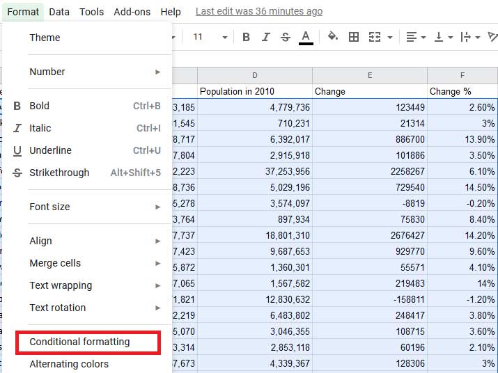

A conditional formatting toolbar will pop up on the right side of your screen.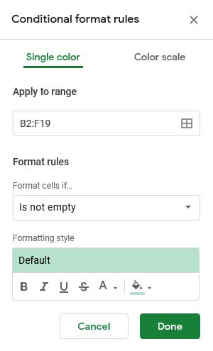

Select the range of cells you want to format. You can also add multiple ranges by clicking the icon to the right of the range field and selecting Add another range. After entering the range, click on ok.

Under Formatting style, click Default, and you'll see the default styling options.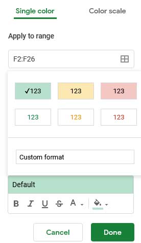

If none of these options are what you're looking for, you can create a custom style, and doing so is no different from selecting your style for anything else in a spreadsheet. You can choose for the text style to be bold, italics, underline, or strikethrough, and you can select your font color and cell background color.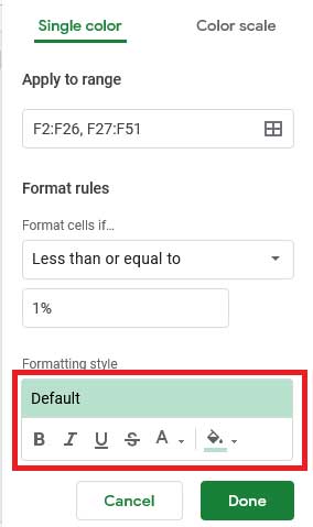

For this example, we will turn the cells green according to conditions.
For the If clause, you can choose if the cell is empty/not empty.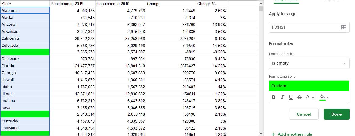

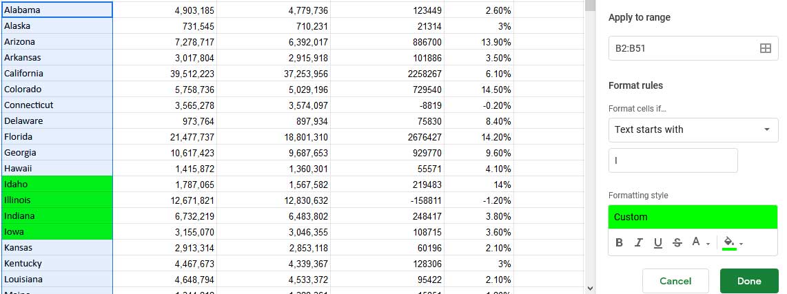
With a text-based rule, a cell will change based on what text you type into it. And you can trigger off of a variety of options, based on the following clauses:

• Text contains
• The text does not contain
• Text starts with
• Text ends with
• Text is exactly

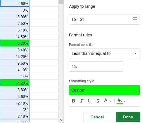
If you want to trigger conditional formatting based on numbers, you have eight options:

• Greater than
• Greater than or equal to
• Less than
• Less than or equal to
• Is equal to
• Is not equal to
• Is between
• Is not between

For date-based conditional formatting, you have three options:

• Date is
• Date is before
• Date is after

Conditional Formatting can be a great tool for businesses to analyze the data they want based on specific criteria and their requirements. With workflow automation, you can receive the results of the conditional formatting in other tools as well. Now that you understand the basics of conditional formatting, you can integrate Google Sheets with 150+ apps through Appy Pie Connect. This Google Sheets-Appy Pie Connect integration can help users integrate your google sheets with various apps without writing a single line of code.